Section 6 Erosion pins
6.1 Dataset Building
6.1.1 Extracting elevation, slope, and curvature from DEMS to GPS points.
Import GPS data points saved in the G-drive (collected using Field Maps and downloaded through Arc Online). Transform into NAD83 zone 15N.
# load erosion pin points,
arb_gps_raw <- read.csv("C:/Users/natha/Documents/local_data/_data/_erosion_pins/_transect_gps/Erosion_Pin_Transects_1.csv") %>%
  select(Latitude, Longitude) %>%
  filter(Latitude < 45) # arb and lr are in the same file, split into 2

lr_gps_raw <- read.csv("C:/Users/natha/Documents/local_data/_data/_erosion_pins/_transect_gps/Erosion_Pin_Transects_1.csv") %>%
  select(Latitude, Longitude) %>%
  filter(Latitude > 45)

# above points are theoretically in WGS84. this tells r they are (which in R the crs is EPSG: 4326). this also makes them a simple features feature (sf)
arb_gps <- st_as_sf(arb_gps_raw, coords = c("Longitude", "Latitude"), crs = 4326)
lr_gps <- st_as_sf(lr_gps_raw, coords = c("Longitude", "Latitude"), crs = 4326)

# transform from WGS84 to NAD83 zone 15N to match lidar (EPSG: 4269)
arb_NAD <- st_transform(arb_gps, crs = 26915)
lr_NAD <- st_transform(lr_gps, crs = 26915)

lr_NAD <- lr_NAD[-31,] # remove junk point
Import dems from drive (created in 26_mapping).
# lr
lr_1m_dem <- rast("C:/Users/natha/Documents/local_data/_data/_mapping/_lake_rebecca_topo/lr_1m_dem")
lr_1m_slope <- rast("C:/Users/natha/Documents/local_data/_data/_mapping/_lake_rebecca_topo/lr_1m_slope")
lr_1m_curvature <- rast("C:/Users/natha/Documents/local_data/_data/_mapping/_lake_rebecca_topo/lr_1m_curvature")

# arb
arb_1m_dem <- rast("C:/Users/natha/Documents/local_data/_data/_mapping/_arb_topo/arb_1m_dem")
arb_1m_slope <- rast("C:/Users/natha/Documents/local_data/_data/_mapping/_arb_topo/arb_1m_slope")
arb_1m_curvature <- rast("C:/Users/natha/Documents/local_data/_data/_mapping/_arb_topo/arb_1m_curvature")
Extract elevation, slope, and curvature (in 1/m) at gps points.
# arb
arb_NAD$elevation <- terra::extract(arb_1m_dem, arb_NAD)[,2]
arb_NAD$slope <- terra::extract(arb_1m_slope, arb_NAD)[,2]
arb_NAD$curvature <- terra::extract(arb_1m_curvature, arb_NAD)[,2]

# lr
lr_NAD$elevation <- terra::extract(lr_1m_dem, lr_NAD)[,2]
lr_NAD$slope <- terra::extract(lr_1m_slope, lr_NAD)[,2]
lr_NAD$curvature <- terra::extract(lr_1m_curvature, lr_NAD)[,2]
Export data sets to drive.
# export as shape files (.shp)
write_sf(arb_NAD, "C:/Users/natha/Documents/local_data/_data/_erosion_pins/_arb_geo_data_shp/arb_geo_data.shp")
write_sf(lr_NAD, "C:/Users/natha/Documents/local_data/_data/_erosion_pins/_lr_geo_data_shp/lr_geo_data.shp")

# export as tables (.csv)
write.csv(arb_NAD, "C:/Users/natha/Documents/local_data/_data/_erosion_pins/arb_geo_data.csv", quote = 1)
write.csv(lr_NAD, "C:/Users/natha/Documents/local_data/_data/_erosion_pins/lr_geo_data.csv", quote = 1)
6.2 Visualizing etc.
6.2.1 Spatial Plots
Import GPS and dem data.
# import shape files
arb_geo_shp <- read_sf("C:/Users/natha/Documents/local_data/_data/_erosion_pins/_arb_geo_data_shp/arb_geo_data.shp")
lr_geo_shp <- read_sf("C:/Users/natha/Documents/local_data/_data/_erosion_pins/_lr_geo_data_shp/lr_geo_data.shp")

# import elevation slope curvature data
arb_geo_data <- read.csv("C:/Users/natha/Documents/local_data/_data/_erosion_pins/arb_geo_data.csv")
lr_geo_data <- read.csv("C:/Users/natha/Documents/local_data/_data/_erosion_pins/lr_geo_data.csv")

# merge two above
arb_geo_data[1:2] <- st_coordinates(arb_geo_shp)
arb_geo_data <- rename(arb_geo_data, "latitude" = X, "longitude" = geometry)

lr_geo_data[1:2] <- st_coordinates(lr_geo_shp)
lr_geo_data <- rename(lr_geo_data, "latitude" = X, "longitude" = geometry)

# dems
lr_1m_dem <- rast("C:/Users/natha/Documents/local_data/_data/_mapping/_lake_rebecca_topo/lr_1m_dem")
lr_1m_slope <- rast("C:/Users/natha/Documents/local_data/_data/_mapping/_lake_rebecca_topo/lr_1m_slope")
lr_1m_curvature <- rast("C:/Users/natha/Documents/local_data/_data/_mapping/_lake_rebecca_topo/lr_1m_curvature")

arb_1m_dem <- rast("C:/Users/natha/Documents/local_data/_data/_mapping/_arb_topo/arb_1m_dem")
arb_1m_slope <- rast("C:/Users/natha/Documents/local_data/_data/_mapping/_arb_topo/arb_1m_slope")
arb_1m_curvature <- rast("C:/Users/natha/Documents/local_data/_data/_mapping/_arb_topo/arb_1m_curvature")
Plotting fun
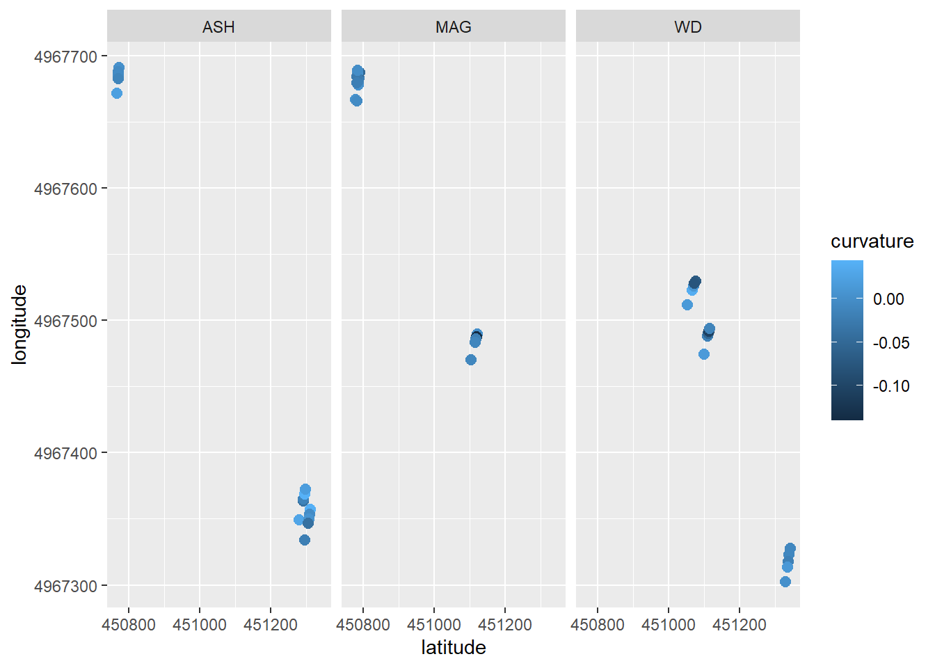
arb_geo_data$site = NA
arb_geo_data[1:15,]$site = "ASH"
arb_geo_data[16:30,]$site = "MAG"
arb_geo_data[31:45,]$site = "WD"

ggplot(arb_geo_data, mapping = aes(latitude, longitude, group = site, color = curvature)) +
  geom_point(size = 2.5) +
  facet_wrap(~site)